Early computers were constructed using vacuum tubes and ran inconsistently at the best of times, with tubes failing on average every two days (Randall 2006). One such early computer was named ILLIAC, and was used by professor Lejaren Hiller at the University of Illinois to compose what is generally regarded as the first computer generated piece of music, the Illiac Suite (Zipris n.d.). Quantum computers of today are at a similar level of development: they are bulky, expensive, fragile, and limited in terms of computational power. Current classical computers are still generally computationally advantageous to use over quantum computers, but that is expected to change over the next several years as both the size and quality of quantum computers improve (Lanes, et al. 2025).

With the advent of quantum computation, new types of calculations will soon become accessible to scholars and artists. For example, simulation of quantum systems will be easier to calculate using an inherently quantum mechanical system, an application which was pointed out when Richard Feynman first posed the idea of a quantum computer (Feynman 1981). This includes problems like the protein folding problem, an issue fundamental to modern cancer research (Ramesh/ Tomesh/ Riesenfeld/ Chong/ Pearson 2024). Quantum computers are also particularly good at solving optimization problems (Moll, et al. 2018). One such example is that of the traveling salesperson which asks: if a salesperson must travel between X cities throughout a region, what route uses the least amount of fuel? Optimization problems crop up in several fields including global economics, supply logistics, many areas of science, cryptography, and so forth. The breadth in application of these devices has led the US government to consider the development and understanding of this technology a matter of national security (The White House 2022).

Comparatively little thought has been given to artistic applications of quantum computers. Thanks primarily to the efforts of Eduardo Reck Miranda and the International Symposium on Quantum Computing and Musical Creativity, there is a small collection of writing on the topic of quantum computation and music (OCH/ Itaborala 2025). As a field, quantum computer music is less than a decade old, and there are many fundamental questions about the applicability of this technology for music creation and dissemination that have not been broached. It could turn out that quantum computers are never going to be accessible in a practical way. On the other hand, a handful of significant breakthroughs could pave the way for an unprecedented change to our computational abilities, partially due to the dramatic improvements in AI that are anticipated as quantum computers are integrated into the training process (Acampora/ Chiatto/ Schiattarella/ Vitiello 2026). With seemingly exponential progress in the development of quantum computational hardware, now is the time to give more thought to the software side of quantum computation: quantum algorithms. This paper serves to broaden the accessibility of quantum computation by providing a path towards hands-on utilization of the devices for the sake of music creation.

In the following, I take a pedagogical approach to the topic of quantum computation aimed at readers with limited training in mathematics or physics, but perhaps some experience in digital signal processing. This article begins with an introduction to qubits and linear algebra before describing original quantum algorithms which can be used to process audio signals. Not all these algorithms will necessarily be faster than their classical counterparts. In fact, due to the simple audio encoding scheme used in this paper, several of them are slower. Nevertheless, these basic quantum audio effects are intended to provide a conceptual basis for the reader to understand simple quantum algorithms. The value of these examples lies not in their computational efficiency, but rather in their ability to illustrate fundamentals of quantum computing. In this paper, I use under-sampling, block-encoding, and convolutional algorithms to produce several audio effects including distortion, filtering, and reverb.

  Introduction to Quantum Computation

In the following, I present a brief introduction to quantum computing that is designed to be accessible to readers with a basic understanding of matrix algebra and digital signal processing, but perhaps no familiarity with the specific notation of quantum physics and computation. For a more detailed introduction at a similar level of mathematical rigor, I recommend consulting the text Quantum Computing for Everyone by Chris Bernhardt (Bernhardt 2019). Though it is not necessary for comprehending this paper, a more detailed overview of quantum mechanics can be found in the undergraduate text by Griffiths (Griffiths/ Schroeter 2018) and the graduate text by Sakurai (Sakurai/ Napolitano 2011), among others. The seminal text by Nielsen and Chuang (Nielsen/ Chuang 2000) on quantum computing is also exceptionally useful for those wishing to pursue any aspect of quantum computing at a deep level.

Superposition
Just as the fundamental computational unit in our everyday classical computers is a bit, there is a quantum analog for quantum computers called a qubit. Just like a bit, a qubit has two states in which it can exist: 0 and 1. The difference is that while in the midst of a calculation, the qubit can exist in a superposition of both the states 0 and 1. At the end of a calculation, the state of the qubit will be measured as either 0 or 1, the probability of each outcome dependent on how much of each basis state is present in the superposition.

Superposition is a concept we encounter in music all the time; if two sine waves are each played through a pair of speakers at sufficiently different frequencies, they superimpose in the air, and we may hear them in our ears as a diad. The difference in a quantum mechanical setting is that rather than hearing a diad, the superposition collapses into a single tone as our eardrum measures the wave, more often the louder of the two, and we would hear only a single tone in this quantum mechanical thought experiment.

In modern digital computers, the bit manifests in the transistor. In the quantum realm, however, there are many competing hardware realizations of the qubit. There are several properties of quantum systems which can exist in a superposition of multiple states that would be appropriate for creating a qubit. An understanding of the physical implementation of the qubit, however, is not necessary to follow the mathematics presented below. At any rate, there are too many competing physical realizations of the qubit to adequately detail them all. (Nielsen/ Chuang 2010)

Linear Algebra
The specific mathematical language of quantum computation is linear algebra. In addition to common mathematical operations like addition, subtraction, and multiplication, linear algebra provides a further level of abstracted operations which can act on vectors. A vector is simply a list of numbers, each number corresponding to a dimension. In physics vernacular, the state of a quantum system is a vector called a ket and denoted by |ψ⟩ where ψ is a label for the state in question.

Suppose there is a single bit of information. The quantum computing convention is to write the basis states |0⟩ and |1⟩ as matrices in the form

$ | 0 ⟩ = \begin{bmatrix} 1\\0 \end{bmatrix} and   | 1 ⟩=\begin{bmatrix} 0\\1 \end{bmatrix}. $

Any two matrices can be multiplied together so long as the number of columns in the first matrix is equal to the number of rows in the second matrix. As an example, the multiplication of a pair of 2X2 square matrices is given by the following.

$ \begin{bmatrix} \alpha_{1} & \beta_{1} \\ \gamma_{1} & \delta _{1} \\ \end{bmatrix} \begin{bmatrix} \alpha_{2} & \beta_{2} \\ \gamma_{2} & \delta _{2} \\ \end{bmatrix} = \begin{bmatrix} \alpha_{1} \alpha_{2} + \beta_{1} \gamma _{2} & \alpha_{1} \beta_{2} + \beta_{1} \beta_{2} \\ \gamma_{1} \alpha_{2} + \delta_{1} \gamma _{2} & \gamma_{1} \beta_{2} + \delta _{1} \delta _{2} \\ \end{bmatrix} $

Say we want to create a matrix by which we can multiply the state |0⟩ and produce the state |1⟩ or vice-versa. Such an operation models a NOT gate, labeled here as N. Operators, just like the states mentioned previously, can be represented using a matrix. Using the operator N to act on |0⟩ can be worked out in the following way:

$ N|0⟩= \begin{bmatrix} 0 & 1 \\ 1 & 0 \\ \end{bmatrix} \begin{bmatrix} 0 \\1 \end{bmatrix}= \begin{bmatrix} 0×1+1×0 \\1×1+0×0 \end{bmatrix}= \begin{bmatrix} 0 \\1 \end{bmatrix}= | 1 ⟩ $

There are some interesting quantum effects that can be observed using only a single qubit, but to fully utilize a quantum computer, there must be some way to represent more than one qubit at a time. Whenever a new qubit is added to the computation, the number of possible output states doubles. The conventional way to create a multi-qubit state is to use the tensor product, denoted by ⊗. Taking the tensor product between two single-qubit states produces a four-dimensional state in the following way:

$ \begin{bmatrix} \alpha _{1}\\\beta _{1} \end{bmatrix}\bigotimes \begin{bmatrix}\alpha _{2}\\\beta _{2} \end{bmatrix}= \begin{bmatrix} \alpha _{1} & \begin{bmatrix} \alpha _{2} \\\beta _{2} \end{bmatrix} \\ \beta _{1}& \begin{bmatrix} \alpha _{2} \\\beta _{2} \end{bmatrix} \\ \end{bmatrix} = \begin{bmatrix} \alpha _{1}\alpha _{2} \\ \alpha _{1}\beta _{2} \\ \beta _{1}\alpha _{2}\\ \beta _{1}\beta _{2} \end{bmatrix} $

All the operators that appear in quantum computing are square, which is to say the number of rows in the matrix is equal to the number of columns. One important property of these square matrices is unitarity, which means that they are invertible, or in other words, any series of quantum operations can be reversed. This is distinct from the digital case, where information is lost after applying some logic gates. For example, the OR gate returns 0 when both inputs are 0, but 1 otherwise. If I had only knowledge about the output state, I could figure out the input states in the case I measure 0, but if I measure 1, I have no idea what the inputs were. An OR gate is not unitary, which means it cannot be directly implemented on a quantum computer.

Any matrix that is unitary can be decomposed into a series of logic gates and run on a quantum computer. For a matrix to be unitary, it must be square and obey

$ \textit{U}^{\dagger}\textit{U}= \textit{UU}^{\dagger}= \textit{I}, $

where I is an identity matrix and † (pronounced dagger) represents a Hermitian adjoint. An identity matrix is one where each diagonal element (i.e. a matrix element whose row and column indices are equal) is 1, and all other elements are 0. For example, here is a 2X2 identity matrix.

$ \textit{I}= \begin{bmatrix} 1 & 0 \\ 0 & 1 \\ \end{bmatrix} $

Taking the Hermitian adjoint of a matrix just means that the matrix is transposed, and the complex conjugate is taken. To find a complex conjugate is simple: just flip the sign of the imaginary part of a complex number. To find the transpose of a matrix, swap the row and column indices of each matrix element. Below is an example calculation of the Hermitian adjoint of a general 2X2 matrix.

$ \textit{A}= \begin{bmatrix} \alpha _{r}+ i\alpha _{i}& \beta _{r}+i\beta _{i} \\ \gamma _{r}+i\gamma _{i}& \delta _{r}+i\delta _{i} \\ \end{bmatrix} $
$ \textit{A}^{\dagger}= \begin{bmatrix} \alpha _{r}- i\alpha _{i}& \gamma _{r}-i\gamma _{i} \\ \beta _{r}-i\beta _{i}& \delta _{r}-i\delta _{i} \\ \end{bmatrix} $

Matrix multiplication, the tensor product, and the notion of unitarity are all we need from linear algebra to construct a variety of simple quantum signal processing algorithms. One additional mathematical operation is needed for some of the more advanced calculations in this paper called block encoding, also sometimes referred to as unitary dilation or qubitization (Low/ Chuang 2019).

Sometimes, it may be desirable to perform a non-unitary matrix operation on a quantum computer, which is not allowed. Block encoding is any method of embedding a non-unitary matrix as a component within a larger unitary matrix which can be decomposed and run on a quantum computer without issue. Consider a non-unitary matrix A. While A cannot directly operate on a set of qubits, a unitary matrix U can be proposed which contains A of the form

$ \textit{U}= \begin{bmatrix} A & * \\ * & * \\ \end{bmatrix}, $

where the asterisks indicate computationally irrelevant matrix areas which must be constructed to maintain unitarity. The most general way to find U is by calculating

$ \textit{U}= \begin{bmatrix} A & \sqrt{I-AA^{\dagger }} \\ \sqrt{I-AA^{\dagger }} & A \\ \end{bmatrix}, $

though more efficient calculations can be done for certain structures of A. The result of this unitary dilation is that a square matrix with d rows and d columns has been rewritten into something computationally useful that has 2d columns and 2d rows.

Qubits and Quantum Logic Gates
Suppose a qubit is in the state

$ |+⟩=\frac{1}{\sqrt{2}}\begin{bmatrix} 1 \\1 \end{bmatrix}, $

or in other words, an equal superposition of the states |0⟩ and |1⟩. The first question one might have is: why is there a factor of 1/$\sqrt{2}$ in front of the matrix? The reason has to do with measurement: the probability of measuring a particular basis state of |+⟩ is equal to the corresponding value in the matrix, squared. When the system is measured, something must be measured, so the probabilities of each measurement should add up to 1. In this case, 1/$\sqrt{2}$ can be squared to get one half, and two halves add up to 1, so there is a 100 percent chance that something will be measured, and there is a fifty percent chance of that value being 0 and a fifty percent chance of that value being 1. The process of finding the factor in front of the matrix is called normalization, and a given state is correctly normalized when the sum of probabilities adds to 1.

To create an equal superposition of the basis states, there must be an operation which can transform |0⟩ into |+⟩. One such operation is called a Hadamard gate, and is defined as

$ \textit{H}= \frac{1 }{\sqrt{2}}\begin{bmatrix} 1 & 1 \\ 1 & -1 \\ \end{bmatrix}. $

Letting H operate on |0⟩, the equal superposition state mentioned previously is found and denoted as |+⟩:

$ H | 0 ⟩ = \frac{1}{\sqrt{2}}\begin{bmatrix} 1& 1 \\ 1 & -1 \\ \end{bmatrix} \begin{bmatrix} 1 \\0 \end{bmatrix}= \frac{1}{\sqrt{2}} \begin{bmatrix} 1 \\1 \end{bmatrix}= \frac{1}{\sqrt{2}}$ (|0⟩+ |1⟩) = |+⟩

If the Hadamard gate is applied once again to |+⟩, then |0⟩ is recovered. If the Hadamard gate is instead applied to |1⟩, a minus-sign appears in the new state, so it is represented by |-⟩.

$ H | 1 ⟩ = \frac{1}{\sqrt{2}}\begin{bmatrix} 1& 1 \\ 1 & -1 \\ \end{bmatrix}\begin{bmatrix} 0 \\1 \end{bmatrix}= \frac{1}{\sqrt{2}} \begin{bmatrix} 1 \\-1 \end{bmatrix}= \frac{1}{\sqrt{2}} $ (|0⟩- |1⟩) = |-⟩

One way to visualize the effect quantum gates have on a single qubit is by using the Bloch sphere, a cross-section of which is shown in Figure 1. For the present discussion, a 2-dimensional rendering of the Bloch sphere is sufficient, but a third dimension is required if the quantum state ever involves imaginary numbers. In addition to the Hadamard gate, one more single qubit gate is useful in this paper: the RY gate, which allows rotation of the vector |ψ⟩ in Figure 1 around the Bloch sphere by some angle θ. If a qubit is initialized in the state |0⟩, an RY gate can be applied to the state to rotate it an arbitrary amount. For example, if the vector is rotated by π/2 radians, then the resulting state |+⟩ is identical to the state achieved if a Hadamard gate had been applied instead. If the state is rotated again by the same value, the state |1⟩ is reached.

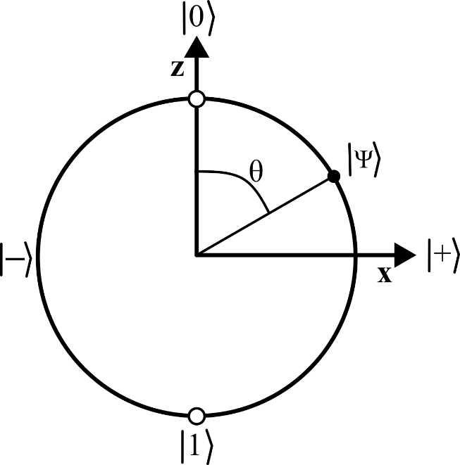
Figure 1. Cross-section view of the Bloch Sphere. The basis states |0⟩ and |1⟩ are found at the top and bottom of the diagram respectively. The equal superposition states |-⟩ and |+⟩ are also shown on the left and right sides of the diagram. An arbitrary qubit state is indicated by |ψ⟩, and is found an angle θ away from |0⟩. Such a state can be achieved by rotating the initialized qubit around the Y-axis, which is protruding into the center of the diagram.

Though I will bypass directly implementing multi-qubit gates in my algorithms in this paper, it is worth describing them because they are essential for decomposing unitary operators into something that can be run on a quantum computer. That decomposition process is well beyond the scope of this paper, but I would be remiss if I did not point out how qubits interact with each other via quantum entanglement.

The simplest and most common multi-qubit gate is the Controlled-NOT gate, often abbreviated to CNOT. In the classical sense, it is a NOT gate that only flips the target bit if some other control bit is in state 1. In a quantum computational setting, it is useful to describe the operation as a matrix of the form

$ \textit{CNOT}= \begin{bmatrix} 1 & 0 & 0 & 0 \\ 0 & 1 & 0 & 0 \\ 0 & 0 & 0 & 1 \\ 0 & 0 & 1 & 0 \\ \end{bmatrix}. $

Given that this operates on two qubits simultaneously, we must first create a two-qubit state for the CNOT gate to operate on. The tensor product can be used to create such a state. As an example, say we take the tensor product between the states |1⟩ and |0⟩:

$ |1⟩ \bigotimes |0⟩=\begin{bmatrix} 0 \\1 \end{bmatrix}\bigotimes\begin{bmatrix} 1 \\0 \end{bmatrix}= \begin{bmatrix} 0 & \begin{bmatrix} 1 \\0 \end{bmatrix} \\ 1 & \begin{bmatrix} 1 \\0 \end{bmatrix} \\ \end{bmatrix}= \begin{bmatrix} 0 \\ 0 \\ 1 \\0 \end{bmatrix} $

Allowing the CNOT gate to operate on this state, (which I will abbreviate as |10⟩), it can be observed that the values in the two last rows have been flipped.

$ CNOT|10⟩=\begin{bmatrix} 1 & 0 & 0 & 0 \\ 0 & 1 & 0 & 0 \\ 0 & 0 & 0 & 1 \\ 0 & 0 & 1 & 0 \\ \end{bmatrix}\begin{bmatrix} 0\\ 0\\ 1\\0 \end{bmatrix}= \begin{bmatrix} 0\\ 0\\ 0\\1 \end{bmatrix} =|11⟩ $

Note that the combined state |0⟩⊗|1⟩ is distinct from |1⟩⊗|0⟩, and the CNOT gate will behave differently when made to operate on these states.

Quantum Circuit Diagrams
Much as circuit diagrams can be used to show the organization of resistors and capacitors in analog circuits or NAND gates and NOT gates in digital circuits, quantum circuit diagrams can be used to represent all the gate operations mentioned so far and many more. The anatomy of a quantum circuit diagram is remarkably simple: each qubit required for a calculation is represented by a horizontal line. Qubit operations appear left to right on the diagram in the order which they affect the qubit or qubits. Single qubit operations appear as boxes on the corresponding qubit, and controlled operations extend a vertical line towards the corresponding control qubit. Figure 2 shows a diagram containing a Hadamard gate and a CNOT gate being used to create a special state called a Bell state. The significance of the Bell state is beyond the scope of this paper, but in short, this is the simplest circuit one can create to produce a pair of quantum entangled qubits. The CNOT gate is somewhat unique in that it does not typically manifest in a quantum circuit diagram as a box with a line, but rather a pair of circles on the control and target qubits.

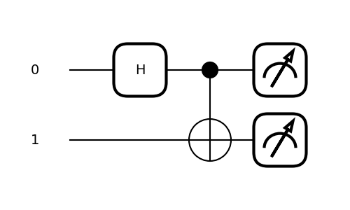
Figure 2. Quantum circuit diagram depicting a series of gates which can be used to create a Bell state. A Hadamard gate is first applied to qubit 0 before it becomes the control qubit in a CNOT gate across qubits 0 and 1. The states of both qubits are measured at the end of the calculation.

Multi-qubit operations, such as the unitary operation appearing in Figure 9, appear as a box spanning multiple qubits. These unitary gates typically hide a complex decomposition of rotation and CNOT gates. At the beginning of a quantum circuit on the left-hand side there are often a collection of zeros representing the initial state of the qubits before computation, and a bespoke measurement symbol is applied at the end of the circuit to the relevant qubits. Though the mathematics behind some of the effects presented in this paper may be challenging to digest at first glance, I hope that by providing clear circuit diagrams I can show that the operations required to achieve the effect are remarkably few.

Why Use a Quantum Computer?
Many of the algorithms presented in this paper are readily achievable using digital and/or analog hardware. A logical question then arises: why bother to re-implement these processes on quantum hardware? I have two answers to this question. The first is speed; an exceptional amount of funding has been directed towards quantum computing research because of just how much faster they are than classical computers at solving a few important problems. Though the emphasis in this paper is not computational efficiency, the broader field of quantum algorithms is driven by the search for speed advantages over digital computers. For example, Grover’s search algorithm is useful for efficiently searching databases with N number of entries, and allows you to find what you’re looking for in the order of $\sqrt{N}$ steps (often abbreviated as $O\sqrt{N}$ steps), whereas a classical search algorithm is much slower, taking $O(N) $ steps (Grover 1996). An even more dramatic speedup is found using Shor’s algorithm discovered in 1995 to factor large numbers into their prime factors (Shor 1999).

There is potential for known digital signal processing algorithms to be executed much more efficiently using quantum hardware. There are some known algorithms, such as the Finite Impulse Response (FIR) filter described later in this paper, which can be computationally cumbersome on digital computers, but may one day be reasonably accessed using quantum computers. It also turns out that some of the most important quantum algorithms are unified by the notion of quantum signal processing, the very same framework I use later in this paper (Martyn/ Rossi/ Tan/ Chuang 2021).

My second motivating factor has to do with the creative implications of quantum computing and audio. There are several moments in the history of music where a new technology gave musicians a new method of expression. The advent of analog synthesis provided radically different tools for the creation of music than anything seen before. The technical limitations and new ways of representing audio in digital hardware further expanded the range of signal processing techniques into a new expressive domain. Quantum computing is still young, but I believe such a fundamental shift in how computers work is fertile ground for the development of new tools for musical expression.

  Single-Qubit Audio Encoding

It is possible to encode a single sample of audio up to an arbitrary level of precision using only a single qubit. The key to encoding audio into a quantum system is normalizing the audio to fit within a range of rotation angles between 0 and π, corresponding to state vector angles in the right hemisphere of the Bloch sphere in Figure 1. Once the rotation angle θ is known, the qubit can be rotated to the desired position, and the sample is encoded! A single rotation gate about the Y-axis is required to encode a single sample of audio into a quantum computer using this method, as shown in Figure 3.

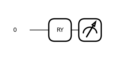
Figure 3. Quantum circuit diagram depicting a single-qubit audio encoding and decoding scheme. A qubit is initialized in state |0⟩, then rotated about the Y-axis depending on the amplitude of the audio sample. In this simple case, the sample is measured without further processing.

Programming libraries exist which can take an audio sample and represent it as a float – I used the python package audioio in my own experimentation. Given an audio sample s represented as a float between -1 and 1, the encoding angle is given by

$ \theta =\frac{\pi }{2}\left ( s+1 \right ). $

After a single measurement, the quantum computer will return either 1 if the state |0⟩ is measured or -1 if the state |1⟩ is measured. After a specified number of measurements (often called shots), the average measurement M is returned to the user, a value between -1 and 1. The measurement we get back, however, is not the audio signal but related trigonometrically to the audio signal. To invert the trigonometric relationship between the qubit rotation angle and the probability of measuring |0⟩, or |1⟩, and thereby rebuild the measured audio signal m, I have employed the following formula:

$ m = 1-\frac{4}{\pi } arcsin\left ( \sqrt{\frac{M+1}{2}} \right ) $

Figure 4 depicts the mapping between five samples and five qubits. Samples valued greater than 0 appear in the upper-right quadrant of the qubit, while samples valued less than 0 appear in the bottom-right quadrant of the qubit.

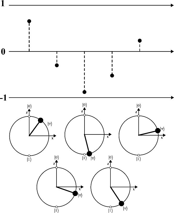
Figure 4. Sketch depicting the relationship between individual samples and their single qubit encodings. Each sample in the top half of the figure corresponds to a Bloch circle at the bottom of the figure. Higher amplitude samples are mapped closer to the basis states |0⟩ and |1⟩, while lower amplitude samples are mapped closer to the positive equal superposition state. Values and angles shown are approximate.

Although it is simple to encode an audio sample into a single qubit, retrieving the information after processing is not so straightforward. To retrieve the information from the system, the state must be measured repeatedly to reconstruct the encoded sample. If an 8-bit sample is encoded into the qubit, then a minimum of 8 measurements are theoretically needed for reconstruction, but the randomness inherent in the measurement means that hundreds or thousands of measurements are more likely to be needed. To measure the qubit is like flipping a weighted coin, and after measuring many times, there may be a slight difference between the encoded and decoded signals, even after many more measurements than technically required to reconstruct the signal.

It may seem as though the probabilistic nature of this encoding and decoding scheme is so inefficient as to be impractical. Though it would take some time to do many measurements using a single qubit, the computation time drops significantly if the measurements could be done in parallel. IBM boasts a quantum computing architecture named Condor which features a quantum processor with 1121 superconducting qubits (AbuGhanem 2025), and the company is on track to rapidly increase their quantum computing capabilities within the next few years (Angelini/ Forgione 2025). Today, 8-bit audio can be encoded and probabilistically retrieved at a more than reasonable bit-depth using a single parallel calculation spanning over one hundred qubits.

The second reason this method of audio encoding is worth pursuing is for its conceptual simplicity. There are methods of encoding audio in a quantum system which use exponentially fewer qubits, but given the pedagogical nature of this paper, I believe this single qubit encoding scheme is worth investigating as a simple toy model. At any rate, quantum audio signal processing research is in its infancy, it could very well be the case that this encoding scheme has significant advantages over other seemingly more efficient schema.

  Quantum Audio Processing Algorithms

I have briefly presented all the tools necessary to begin exploring audio signal processing methods using a quantum computer. In the following, I introduce effects processes that resemble bit crushing, wave folding, soft clipping, filtering, and reverb.

Qubit Crushing
Due to the probabilistic nature of retrieving audio from the quantum system, there is an opportunity to produce an interesting effect by under-sampling the system. There is a method of digital signal processing which is guided by a similar principle called bit-crushing. To bit-crush audio, a higher bit-depth sample is under-represented at a lower bit-depth. For example, a 24-bit audio sample could be approximated using 8-bits to obtain a chiptune-style sound. Similarly, if I reduce the number of measurements used to retrieve the information from the qubit, the sound is degraded in what may be an interesting or useful way.

Under-measuring the system may be the simplest way to process sound using our single qubit quantum audio encoding scheme. Simply encode the audio, then measure it fewer times than required to accurately retrieve the audio. The result is a sound which has more noise as fewer measurements are taken as shown in Figure 5. The noise introduced to the signal follows the contour of the input. Perceptually, I feel that the resulting sound is distinct from the masking effect that usually happens when noise is layered onto a signal. Using this qubit crushing procedure in an artistic way, a precise number of measurements could be found which adds noise to the signal while minimally masking the pitch and timbre characteristics of a sound.

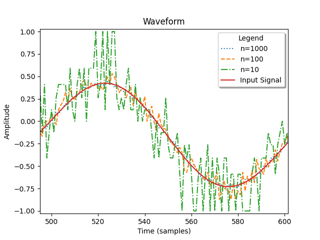
Figure 5. Plot of qubit-crushed samples for multiple numbers of measurements given by n. An input signal denoted by a solid line is measured n times. As n increases, the output signal more closely resembles the input. The sonic effect is that a bed of white noise is added to a sound for low n, but the sound is more easily perceptible than if noise were simply layered onto the signal.

It is also worth noting that this noise could be generated without encoding any audio in the first place. By putting a qubit into an arbitrary superposition, a noise signal is generated, implying a possible first step towards a quantum audio synthesis engine.

Sound 1. Unprocessed audio.
Sound 2. Qubit crushed audio recovered using 10 measurements per sample.
Sound 3. Qubit crushed audio recovered using 100 measurements per sample.
Sound 4. Qubit crushed audio recovered using 1,000 measurements per sample.
Sound 5. Qubit crushed audio recovered using 10,000 measurements per sample.

Wave Folding
Because audio information is encoded into a rotation angle about the Y axis of a qubit, to attenuate the signal is to multiply that rotation by some value. The easiest way to perform this multiplication is digitally before the signal is encoded into the quantum system. If an input signal is normalized to the range [-1, 1], gain can be applied before converting the sample to a rotation angle using

$ S=(1+a)s $

where S is the attenuated signal, s is the unattenuated signal, and a is some attenuation value set by the user. The multiplicative factor (1+a) is analogous to gain in a digital or analog setting.

If the attenuation value is set to 0, the signal is unchanged, and values between 0 and -1 attenuate the signal as shown in Figure 6. The attenuation value -1 is functionally equivalent to setting the gain to -∞ on an analog or digital mixer. Lowering the attenuation value beyond -1 however, the signal once again grows in amplitude, though with opposite phase. The attenuated signal amplitude is the same as the input signal when the gain is set to -2.

For input signal values normalized to the maximum possible value, setting the attenuation value greater than 0 or less than -2 causes the signal to be distorted. Rather than signals clipping and squaring off against the upper and lower limits as is often the default in digital signal processing, the waveforms appear to bounce against the boundaries, creating a wave folding effect as shown in Figure 7.

The attenuation control I am manipulating to fold the signal highlights the circular nature of the qubit. When boosting a signal in a digital system, the signal will clip against the upper and lower computational bounds. In this single qubit representation of an audio sample, gain corresponds to a change in rotation of the qubit from the initialized state |0⟩ to the desired value. The wave folding seen in Figure 7 indicates that the folded samples are encoded into the left half of the Bloch circle, unlike any of the Bloch circles depicted in Figure 4.

This quantum method of wave folding is in some ways simpler than an equivalent digital algorithm where the folded components of the waveform are calculated with an algebraic formula. In this narrow version of quantum wave folding, the reflective behavior is built into the nature of the encoding scheme. Rather than accounting for numbers that exceed the amplitude bounds in a digital signal, no additional calculations are required to rotate a quantum audio signal and fold a waveform an arbitrary amount.

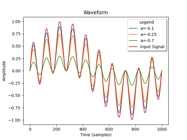
Figure 6. Plot of attenuated signals. Note that when a=0, the input signal is unmodified, and when a=-1, the signal is rendered silent.
Sound 6. Attenuated audio when a=-0.25.
Sound 7. Attenuated audio when a=-0.7.

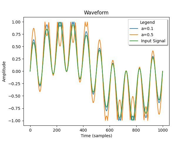
Figure 7. Plot of boosted signals. When a signal is boosted beyond the limits of +/-1, the signal appears to reflect at the boundary and produces a wave folding effect. The greater the value of a, the greater the distortion.
Sound 8. Wave folded audio when a=1.
Sound 9. Wave folded audio when a=2.
Sound 10. Wave folded audio when a=5.

Soft Clipping
Rather than working with one qubit at a time, more interesting effects could be produced by allowing qubits to interact with each other. To create a 2-qubit state where manipulating either of the qubits alters the measurement outcome, we use a tensor product. If an audio sample is encoded into the first qubit and an arbitrary state controlled by the user is encoded into the second qubit, the signal is attenuated in a different way from what I presented in the wave folding example.

I can calculate the tensor product between an encoded audio sample |ψ⟩ and an arbitrary state |α⟩:

$ |\Psi\alpha ⟩ =|\Psi ⟩\bigotimes |\alpha ⟩= \begin{bmatrix} \Psi _{0} \\\Psi _{1} \end{bmatrix}\bigotimes\begin{bmatrix} \alpha _{0} \\\alpha _{1} \end{bmatrix}= \begin{bmatrix} \Psi_{0}\alpha _{0} \\ \Psi_{0}\alpha _{0} \\ \Psi_{1}\alpha _{1} \\\Psi_{1}\alpha _{1} \end{bmatrix}. $

There are four possible measurement outcomes: the state |00⟩ is measured with probability $(\Psi_{0}\alpha _{0} )^{2}$, the state |01⟩ is measured with probability $(\Psi_{0}\alpha _{1} )^{2}$, the state |10⟩ is measured with probability $(\Psi_{1}\alpha _{0} )^{2}$, and the state |11⟩ is measured with probability $(\Psi_{1}\alpha _{1} )^{2}$. I will make the arbitrary decision that when it comes to the recreation of the audio sample I only care about the measured value of the first qubit. The repercussion of this decision is that setting $|\alpha⟩=|0⟩$ and calculating$ |(\Psi \alpha ⟩$ preserves the original signal after measurement.

What if I instead take the tensor product between an audio sample and |+⟩? The result is

$ |\Psi +⟩=\frac{1}{\sqrt{2}}\bigotimes \begin{bmatrix} 1 \\1\end{bmatrix}= \frac{1}{\sqrt{2}}\begin{bmatrix}\Psi _{0} \\ \Psi _{1} \\ \Psi _{0} \\\Psi _{1} \end{bmatrix}. $

The probabilities of measuring |00⟩ and |10⟩ are equivalent, as are the probabilities of measuring |01⟩ and |11⟩. The sonic result is that the signal is entirely attenuated. For user control values between 0 and π/2, signal attenuation is stronger for values closer to π/2 as shown in Figure 8.

The resultant graph is visually striking in its apparent similarity to soft clipping. As the secondary qubit is manually rotated by the user, the higher amplitude samples are attenuated more than the low amplitude samples. This relationship between the two qubits is created using a tensor product, which is an entirely different calculation than the common cubic function commonly used in digital signal processing (Smith 2010).

Sound 11. Soft clipped audio renormalized with angle set to 1.55 radians.
Sound 12. Soft clipped audio renormalized with angle set to 1.55 radians, re-processed five times.

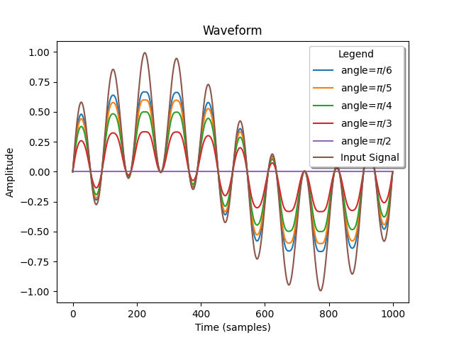
Figure 8. Plot of soft-clipped signals. The input signal is the waveform with the largest amplitude. As the value of the second qubit is changed from 0 to π/2, the signal is compressed such that higher amplitudes are attenuated more than lower amplitudes. The resulting waveform has flatter peaks and resembles the output of a digital soft clipping algorithm. When the second qubit angle is set to π/2 (in other words, an equal superposition of the states |0⟩ and |1⟩), the signal is compressed to silence.

Impulse Response Convolution Filtering A host of digital effects rely on delayed samples called taps. One such effect is a special type of filter called a Finite Impulse Response (FIR) filter which works by convolving a signal with one or more taps coming from that same signal (Smith 2007; Tarr 2018). In the following, I show how to implement such a filter using a quantum computer based on work by Majumdar (Majumdar/ Bakalov/ Baron/ Liu 2025).

The convolved output of a FIR filter can be written as

$ y[n]=\sum_{i=0}^{d-1}P_{i}x[n-i], $

where y is the output state, n is a sample index, d is the number of filter taps, $P_{i}$ is a coefficient at index i determined by the user, and x[n-i] is the input sample at index [n-i]. In the following, I consider only a 3-tap filter, which may be expressed as

$ y[n]=p_{0} x[n]+p_{1} x[n-1]+p_{2} x[n-2]. $

The intent of this formula is to average a sample with two adjacent samples. By carefully selecting values for $P_{i}$ , a high pass filter can be created. To do this on a quantum computer, I will define an input state $|X_{n}⟩$ which contains information about three samples and a normalization coefficient and written as

$ |X_{n} ⟩=\begin{bmatrix} X_{n-2} \\ X_{n-1} \\ X_{n} \\\sqrt{1-X_{n-2}^{2}+X_{n-1}^{2}+X_{n}^{2}} \end{bmatrix}. $

In general, any multi-tap filter can be approximated using a sequence of 1-tap and 2-tap filters. A one tap filter can be cleverly designed by using a non-unitary matrix $F_{1}$ written as

$ F_{1}= \begin{bmatrix} a_{1}/c_{1} & 0 & b_{1}/c_{1} & 0 \\ b_{1}/c_{1} & a_{1}/c_{1} & 0 & 0 \\ 0 & b_{1}/c_{1} & a_{1}/c_{1} & 0 \\ 0 & 0 & 0 & 1 \\ \end{bmatrix}, $

where $a_{1}$ and $b_{1}$ are the feedback and feedforward coefficients, and $c_{1}=\sqrt{a_{1}^{2}+b_{1}^{2}}$. Letting $F_{1}$ operate on the input state, the following state is produced.

$ F_{1}|X_{n} ⟩=\begin{bmatrix} \frac{a_{1}}{c_{1}}x_{n-2}+ \frac{b_{1}}{c_{1}}x_{n} \\ \frac{b_{1}}{c_{1}}x_{n-2}+ \frac{a_{1}}{c_{1}}x_{n-1} \\ \frac{b_{1}}{c_{1}}x_{n-1}+ \frac{a_{1}}{c_{1}}x_{n} \\ \sqrt{1-(x_{n-2}^{2}+x_{n-1}^{2}+x_{n}^{2})} \end{bmatrix} $

The third row of this result is the 1-tap filter. The issue here is that to get this result, the initial state was operated on using a non-unitary matrix, which cannot be done using a quantum computer. The way to get around this restriction is to block encode the non-unitary $F_{1}$ into a larger unitary matrix $U_{1}$.

To generate a unitary matrix which applies a one-tap filter, $F_{1}$ can be encoded in the following way:

$ U_{1}= \begin{bmatrix} F_{1} & \sqrt{1-F_{1}F_{1}^{\dagger }} \\ \sqrt{1-F_{1}F_{1}^{\dagger }}& -F_{1} \\ \end{bmatrix} $

To use this unitary operator, the input state needs padded with zeros to match the number of rows in $U_{1}$ using a tensor product. I will redefine |$X_{n}$ as

$ |X_{n} ⟩= \begin{bmatrix} 1 \\0 \end{bmatrix}\bigotimes \begin{bmatrix} x_{n-2}^{2} \\ x_{n-1}^{2} \\ x_{n}^{2} \\\sqrt{1-(x_{n-2}^{2}+x_{n-1}^{2}+x_{n}^{2})} \end{bmatrix}= \begin{bmatrix} x_{n-2}^{2} \\ x_{n-1}^{2} \\ x_{n}^{2} \\\sqrt{1-(x_{n-2}^{2}+x_{n-1}^{2}+x_{n}^{2})}\\0\\0\\0\\0 \end{bmatrix}. $

If desired, I could calculate $U_{1} |X_{n}$ ⟩ to generate an output $|Y_{n}$ ⟩, but a one-tap filter is so ineffective as to be unnoticeable using my test signal. Instead, I will calculate a three-tap filter, $|Y_{n} ⟩=U_{2} U_{1} |X_{n} ⟩$, which means $U_{2}$ is still needed. The filter I would like to block encode is

$ F_{2}= \begin{bmatrix} 1 & 0 & 0 & 0 \\ 0 & -\frac{a_{2}}{\sqrt{a_{2}^{2}+b_{2}^{2}}} & \frac{b_{2}}{\sqrt{a_{2}^{2}+b_{2}^{2}}} & 0 \\ 0 & \frac{b_{2}}{\sqrt{a_{2}^{2}+b_{2}^{2}}} & \frac{a_{2}}{\sqrt{a_{2}^{2}+b_{2}^{2}}} & 0 \\ 0 &0 & 0 & 1 \\ \end{bmatrix} $

With a matrix of this form, the unitary block-encoded filter can be calculated in a simpler and more efficient way than the 1-tap filter.

$ U_{2}= Z\bigotimes F_{2}= \begin{bmatrix} 1 & 0 \\ 0 & -1 \\ \end{bmatrix}\bigotimes F_{2}=\begin{bmatrix} F_{2} & 0 \\ 0 & -F_{2} \\ \end{bmatrix} $

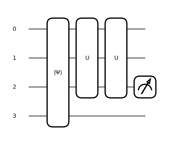
Figure 9. Quantum circuit diagram for a 3-tap FIR filter. The input state is $ |X_{n}$ ⟩ is represented by the general ket |ψ⟩. Two unitary operators act on the first three qubits. The first unitary operator is the one-tap filter $U_{1}$, and the second unitary operator is the two-tap filter $U_{2}$.

For any unitary matrix operation, there exists a decomposition of the operation into fundamental quantum logic gates. Efficiently decomposing unitary gates is an ongoing area of research, so I will instead rely on pre-built algorithms built into several quantum python packages (Cybenko 2001). The unitary matrices $U_{1}$ and $U_{2}$ are 8X8 matrices, which means 3 qubits are needed to execute the operations. As shown in the definition of $ |X_{n}⟩$, however, 4 qubits are needed to encode the input signal. Moreover, only one of the qubits contains the information I want to measure. The result is that the quantum circuit has three ancillary qubits as shown in Figure 9, or in other words three qubits which are not measured but are still required for the calculation. Ancillary qubits appear frequently in quantum computing and can be thought as a sort of “workspace” where computation occurs, but whose output does not carry useful information. The third qubit (labeled 2 in Figure 9) is the one I want to measure. A filtered signal is shown in Figure 10.

The typical digital implementation of a convolutional algorithm grows exponentially as the size of the IR increases, which in this case manifests as the number of taps. Every tap must be multiplied by every sample in the signal. The structure of this quantum convolution, however, implies a less dramatic increase in computational time. Rather than multiplying each number in the IR by each relevant sample, the convolution is handled by single unitary operations. Further study is required to determine what computational advantage there is, if any.

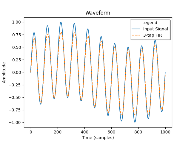
Figure 10. Plot of a signal processed using a 3-tap finite impulse response (FIR) algorithm. The amplitude of the FIR output is approximately ten times smaller than the input and has been scaled here for comparison with the input signal. Note that the filtered signal is shifted two samples to the right of the input signal. The greater deviation between the input and output signals near the extreme amplitudes indicates that the lower frequency component of the waveform has been attenuated, so this is a high-pass filter.

Time Invariant IR Convolution
Another common use of convolution in audio signal processing is reverb. In essence, a time invariant impulse response is combined with some signal, often to emulate the sound of the sample being run through a physical space or hardware. Continuing from the FIR filter of the previous audio effect, I will now consider convolution between two distinct signals.

Suppose there is an audio signal represented in an array as

$ x= \begin{bmatrix} 0 & 0.8 & 0.8 & 0.8 & 0.8 & 0.8 & 0 \\ \end{bmatrix}, $

and a convolution filter stored in a separate array as

$ f= \begin{bmatrix} 0.25 & 0.25 & 0.25 \\ \end{bmatrix}. $

In other words, the audio signal is a square pulse, and I would like to smooth it out by convolving the signal with a shorter pulse at a lower amplitude (Smith 2007). Two signals can be convolved to produce a new signal z by using

$ z(n)=\sum_{m=0}^{n-1}x(m)f(n-m). $

The audio signal can be padded with silence and encoded into the state

$ |X_n ⟩=\begin{bmatrix} 0 \\ x_{4} \\ x_{3} \\ x_{2} \\ x_{1} \\x_{0}\\0\\\sqrt{1-x_{0}^{2}+x_{1}^{2}+x_{2}^{2}+x_{3}^{2}+x_{4}^{2}} \end{bmatrix}. $

I would like to create an operator F which produces the state

$ F|X_{n} ⟩=\begin{bmatrix} f_{0}x_{4} \\ f_{0}x_{3}+f_{1}x_{4}\\ f_{0}x_{2}+f_{1}x_{3}+f_{2}x_{4}\\ f_{0}x_{1}+f_{1}x_{2}+f_{2}x_{3}\\ f_{0}x_{0}+f_{1}x_{1}+f_{2}x_{2}\\ f_{1}x_{0}+f_{2}x_{1}\\ f_{2}x_{0} \\\sqrt{1-(x_{0}^{2}+x_{1}^{2}+x_{2}^{2}+x_{3}^{2}+x_{4}^{2})} \end{bmatrix}. $

Such an operator takes the form

$ F=\begin{bmatrix} 0 & f_{0} & 0 & 0 & 0 & 0 & 0 & 0 \\ 0 & f_{1} & f_{0} & 0 & 0 & 0 & 0 & 0 \\ 0 & f_{2} & f_{1} & f_{0} & 0 & 0 & 0 & 0 \\ 0 & 0 & f_{2} & f_{1} & f_{0} & 0 & 0 & 0 \\ 0 & 0 & 0 & f_{2} & f_{1} & f_{0} & 0 & 0 \\ 0 & 0 & 0 & 0 & f_{2} & f_{1} & 0 & 0 \\ 0 & 0 & 0 & 0 & 0 & f_{2} & 0 & 0 \\ 0 & 0 & 0 & 0 & 0 & 0 & 0 & 1 \end{bmatrix}. $

Just as in the FIR filter case, F can be block encoded to form a unitary matrix U, and the input audio is correspondingly padded with zeros using a tensor product. The difference from the FIR filter case is that I need to produce a matrix of size $2^{7}$=128, where the 7 comes from the number of qubits we want to represent the output signal. This implies inefficiency in our process; the resulting matrix is very sparse and filled mostly with zeros.

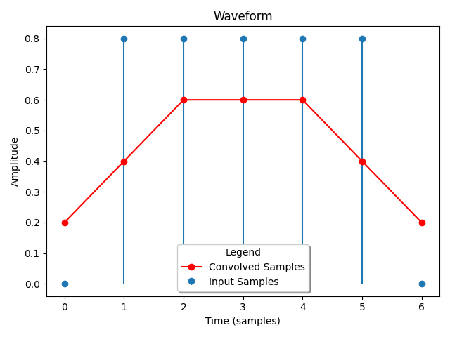
Figure 11. Plot of seven samples before and after convolution. The input signal in blue is convolved with an impulse response consisting of three samples of amplitude 0.25. The result in orange is a “smoothed-out” version of the input pulse. This is the exact same behavior we would expect using a digital convolutional algorithm.

This sort of convolutional algorithm has many common applications in digital signal processing including noise reduction, echo cancellation, reverb, and the FIR filtering seen in the previous section (Christensen 2019). The method of block encoding described in this paper could be expanded to greater numbers of qubits and more complicated effects processes. It is not clear at this stage whether there is a computational advantage when performing these calculations using a quantum computer over a classical computer, but that ambiguity is due mostly to the simple encoding scheme implemented in this paper.

  Conclusion

In this paper, I have introduced five audio effects processing techniques: qubit crushing, wave folding, soft clipping, impulse response convolution filtering, and time invariant impulse response convolution.

Qubit crushing has no perfect digital or analog parallel, so it is difficult to say whether qubit crushing on a quantum computer is or is not computationally advantageous over an aesthetically similar approach, for example layering a sound with additional noise in a digital or analog system. Soft clipping on a digital system is calculated using a stepwise function for each sample, and computation time grows linearly with the number of samples exactly like this quantum algorithm. The same can be said of the wave folding algorithm, though it is arguably more idiomatic to implement a quantum wave folding algorithm than a digital or analog one.

The convolutional algorithms presented are faithful recreations of their digital counterparts. It is possible that this quantum convolutional approach is faster than a digital approach, but more study is needed. To ensure there is a computational advantage when using quantum computers to process audio, a more efficient audio encoding scheme is required.

Future Work

The next direction of research I will pursue involves a fundamental redesign of the audio encoding methodology. It is apparent from several of the large and rather sparsely populated unitary matrices presented in this paper that there is room for more efficient calculation. To expand the speed of computation, the first step is to figure out a more efficient and versatile way of encoding audio.

One could design an audio encoding scheme which represents exponentially more samples while the number of qubits grows linearly. For example, if a system has three qubits, then there are 8 possible states which could be measured, each with their own probability. Just as a single audio sample was encoded into a single qubit in this paper, four samples could be represented using 3 qubits. The general formula for the number of encoded samples would be $2^{n-1}$ where n is the number of qubits. With a mere 100 qubits, $6.33×10^{29}$ samples could be represented, which is about 104 quadrillion ($10^{15}$) years of 192kHz audio, a duration many times longer than the age of the universe. Quantum processors of this size already exist today. Of course, extracting the audio after such an encoding may prove challenging. This alternative multi-qubit encoding scheme also makes a useful algorithm available to us called the quantum Fourier transformation, allowing the exploration of frequency domain effects processes.

There is much promise in the method of block encoding covered in this paper, and I believe it is likely that many signal processing routines could be implemented with a cleverly designed unitary operator. One clear path forward for this research is to simply continue attempting to implement known digital and analog effects processes in the form of a unitary operator acting on a sequence of qubits.

I briefly mentioned while describing qubit crushing that measuring a qubit in an equal superposition of the basis states returns a random number and generates noise. There are other simulations and calculations idiomatic to quantum computers which could prove useful waveform generators. For example, there are physical systems which experience interesting dynamic behavior that could generate audio examples. In the study of quantum phase transitions, it is common to consider a situation where some interaction between particles is activated, and the system is allowed to evolve. This is a study of quantum quench dynamics, it is readily simulated using a quantum computer, and it may produce an interesting sound with the correct mapping.

Taken together, these new implementations of extant audio effects processes represent the first steps towards a conceptual bridge between audio signal processing and quantum computation. Even a simple one-to-one mapping between sample and qubit allows for a host of processes inspired by and in some cases unique from digital algorithms. This work serves as a starting point for making quantum computation accessible to music technologists through familiar audio processing algorithms and with any luck inspires further research at this specific intersection of audio and quantum computing.

  References

AbuGhanem, M. (2025). IBM quantum computers: evolution, performance, and future directions. The Journal of Supercomputing 81. Retrieved from https://doi.org/ 10.1007/

Acampora, G. / Chiatto, A. / Schiattarella, R. / Vitiello, A. (2026, February). Quantum artificial intelligence: A survey. Computer Science Review 59.

Angelini, E. / Forgione, B. (2025 June 10). IBM Sets the Course to Build World's First Large-Scale, Fault-Tolerant Quantum Computer at New IBM Quantum Data Center. Retrieved from IBM Newsroom: https://newsroom.ibm.com/ 2025-06-10-IBM-Sets-the-Course-to-Build-Worlds-First-Large-Scale,-Fault-Tolerant-Quantum-Computer-at-New-IBM-Quantum-Data-Center

Bernhardt, C. (2019). Quantum Computing for Everyone. Cambridge: The MIT Press.

Christensen, M. G. (2019). Introduction to Audio Processing. Cham: Springer International Publishing.

Cybenko, G. (2001 March-April). Reducing quantum computations to elementary unitary operations. Computing in Science & Engineering 3/ 2: 27-32. doi:10.1109/5992.908999

Feynman, R. P. (1981). Simulating physics with computers. International Journal of Theoretical Physics 21: 467-488.

Griffiths, D. J. / Schroeter, D. F. (2018). Introduction to quantum mechanics (Third edition ed.). Cambridge: Cambridge University Press.

Grover, L. K. (1996). A fast quantum mechanical algorithm for database search. Proceedings of the twenty-eighth annual ACM symposium on Theory of Computing (pp. 212-219). New York: Association for Computing Machinery.

Lanes, O. / Beji, M. / Corcoles, A. D. / Dalyac, C. / Gambetta, J. M. / Henriet, L. / . . . / Peropadre, B. (2025). A Framework for Quantum Advantage. arXiv. Retrieved from https://arxiv.org/abs/2506.20658

Low, G. / Chuang, I. L. (2019). Hamiltonian Simulation by Qubitization. Quantum 163.

Majumdar, A. / Bakalov, B. N. / Baron, D. / Liu, Y. (2025). Implementing Finite Impulse Response Filters on Quantum Computers. ICASSP 2025 - 2025 IEEE International Conference on Acoustics, Speech and Signal Processing (ICASSP) 1-5. doi:10.1109/ ICASSP49660.2025.10887919

Martyn, J. M. / Rossi, Z. M. / Tan, A. K. / Chuang, I. L. (2021). Grand Unification of Quantum Algorithms. PRX Quantum 2/ 4. doi:10.1103/PRXQuantum.2.040203

Moll, N. / Barkoutsos, P. / Bishop, L. S. / Chow, J. M. / Cross, A. / Egger, D. J. / . . . / Temme, K. (2018). Quantum optimization using variational algorithms on near-term quantum devices. Quantum Science and Technology 3/ 3. doi:10.1088/2058-9565/aab822

Nielsen, M. A. / Chuang, I. L. (2000). Quantum computation and quantum information (10th anniversary edition ed.). Cambridge: Cambridge University Press.

Nielsen, M. A. / Chuang, I. L. (2010). Quantum computers: physical realization. In Quantum Computation and Quantum Information: 10th Anniversary Edition (pp. 277-352). Cambridge: Cambridge University Press.

OCH / Itaborala. (2025). ISQCMC Proceedings. Retrieved from ISQCMC International Symposium on Quantum Computing and Musical Creativity: https://isqcmc.org/ Proceedings

Ramesh, S. / Tomesh, T. / Riesenfeld, S. J. / Chong, F. T. / Pearson, A. T. (2024). Quantum computing for oncology. Nat Cancer 5: 811-816. Retrieved from https://doi.org/ 10.1038/s43018-024-00770-9

Randall, A. (2006, February 14). Q&A;: A lost interview with ENIAC co-inventor J. Presper Eckert. Retrieved from Computer World: https://web.archive.org/web/ 20130605100109/http://www.computerworld.com/s/article/108568/Q_A_A_lost_interview_with_ENIAC_co_inventor_J._Presper_Eckert

Sakurai, J. J. / Napolitano, J. (2011). Modern quantum mechanics (Second edition ed.). Boston: Addison-Wesley.

Shor, P. W. (1999). Polynomial-Time Algorithms for Prime Factorization and Discrete Logarithms on a. Society for Industrial and Applied Mathematics Review 41/ 2: 303-332.

Smith, J. O. (2007). Introduction to Digital Filters with Audio Applications: Finite Impulse Response Digital Filters. Retrieved from https://ccrma.stanford.edu/~jos/ filters/Finite_Impulse_Response_Digital.html

Smith, J. O. (2007). Mathematics of the Discrete Fourier Transform (DFT) with Audio Applications, Second Edition: Smoothing a Rectangular Pulse. Retrieved from https://ccrma.stanford.edu/~jos/mdft/Convolution_Example_1_Smoothing.html

Smith, J. O. (2010). Physical Audio Signal Processing: Soft Clipping. Retrieved from https://ccrma.stanford.edu/ ~jos/pasp/Soft_Clipping.html

Tarr, E. (2018). Hack audio : an introduction to computer programming and digital signal processing in MATLAB. London: Routledge.

The White House. (2022 May 4). National Security Memorandum on Promoting United States Leadership in Quantum Computing While Mitigating Risks to Vulnerable Cryptographic Systems. Retrieved from https://bidenwhitehouse.archives.gov/briefing-room/ statements-releases/2022/05/04/national-security-memorandum-on-promoting-united-states-leadership-in-quantum-computing-while-mitigating-risks-to-vulnerable-cryptographic-systems/

Zipris, A. (n.d.). Illiac Suite. Retrieved from Illinois Distributed Museum: https://distributedmuseum.illinois.edu/ exhibit/illiac-suite/

논문투고일: 2025년 09월27일
논문심사일: 2025년 10월24일, 11월19일
게재확정일: 2025년 11월23일